My First Hotdog Detector

Hi there! Welcome back to this series on Deep Learning for image classification. In the two previous installments about imagenet and deep learning, and the train-test split, we managed to get the images we need to build a sweet sweet hotdog/nohotdog classifier using Deep Learning. This time, we are finally going to play around with Convolutional Neural Networks (CNNs)! But wait, what are those???

Neural Networks

The form our classifier is going to take is the Convolutional Neural Network (CNN). These have revolutionized image classification and a lot of other tasks. Remember the 2012 Imagenet challenge?? This is the innovation that changed everyting.

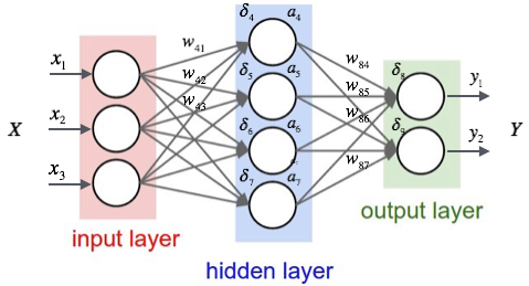
As any other Neural Network, CNNs consist of a series of stacked layers. Each layer consists of a series of neurons. These are simply nodes in a network that hold a floating point value, called their activation. Each node in a layer is connected to the layer immediately below, and the connection has a weight associated with it.

The simplest kind of layer that we can think of is one in which each neuron is connected to all the neurons in the preceding layer. This is called a Dense layer. In it, the activation of each neuron will be calculated from the sum of the activations of every single neuron in the previous layer, each multiplied by the corresponding weight. But that sum is not the activation itself; the activation will be calculated from that sum by applying an activation function.

Weights and activations

Activation functions

As we have just seen, the connection between a neuron and the layer below is shaped by an activation function. This describes the relationship between the values in the preceding layer, the weights, and the activation value. For each neuron its activation $a_i$ will be determined by the expression:

\[a_i = f(\sum_j^n(a_i w_{ij}))\]

That $f$ is the activation function. There are a number of them that can be used without changing terribly how the NN performs. The requisites are basically:

The activation function must be nonlinear. If it was, the whole network would be just a chain of matrix multiplications, and the output would be a linear function of the output. We could save all the trouble and just summarize the whole thing with a single multiplication. And, obviously, it wouldn’t learn anything useful. The fun in NNs is that they are Universal Function Approximators.
The activation function must be differentiable. That is crucial for our gradient descent (remember the last post): we need the derivative, the gradient, to know in what direction we need to push the weights in every step of the optimization.

An early function that was widely used is the logistic function, the same used in logistic regression. If you think about it, then the expression above is exactly logistic regression. Therefore, a neural network can be thought of as a series of logistic regressions stacked one over the other!

In reality, the current most used activation function is the Rectified Linear Unit (ReLu), but at this level the distinction is mostly academic. We don’t need to go into the practical or theoretical differences between the ReLu and the logistic to get a general understanding of how NNs work.

Backpropagation

In logistic regression, we pick the coefficients (corresponding to our weights here) to minimize an error measure given a set of inputs and corresponding outputs. If we had an error measure here, we could adjust the weights so that the error measure for each input is minimized. But we do! it is the difference (measured in any of a number of ways) between the predictions of the network and the true classes. That will work for the last layer.

What about the bottom layers? Well, if we had a perfect last hidden layer, then the previous one would have to predict its activations for a given input. Then, the error measure is the difference between the output of the previous and the “perfect” hidden layer! We can apply this reasoning to adjust the weights of each layer from the top to the bottom (back), for each layer in turn.

Backpropagation is just that! A fancy way of saying: adjust by one step of gradient descent the last layer, then the second-to-last in view of those last layer weights, and so on until you reach the bottom. Rinse and repeat until you are satisfied with the results. This is the breakthrough that made neural networks trainable.

Convolutional Neural Networks

We’ve been talking about neural networks like there was only one kind. However, the recent explosion in Deep Learning performance and width of application is due in no small part to the invention of a variety of network kinds which are especially suited to particular tasks. In our specific application, image classification, and more generally in computer vision the kind that suits us best is the Convolutional Neural Network. This is a network that includes one or more convolutional layers.

A convolutional layer differs from a dense layer in that each neuron in it doesn’t look at the whole layer below it but only to a small region of it, often 3 x 3 or 5 x 5. That means that the first convolutional layer will look at squares of 9 or 25 pixels in much the same way that a neuron in a dense layer looks at its whole input layer. That results first in a huge reduction in number of parameters, which could explode with the kind of input sizes that an image classifier must handle - remember, each pixel in the image will result in three nodes in the input layer! this is a great bonus, but not the main point. The real advantages are:

Translation invariance: a neuron in a convolutional layer will learn to be activated in response to a particular visual feature. It will not care where that feature is: a neuron that recognizes vertical edges will recognize them anywhere in the image.
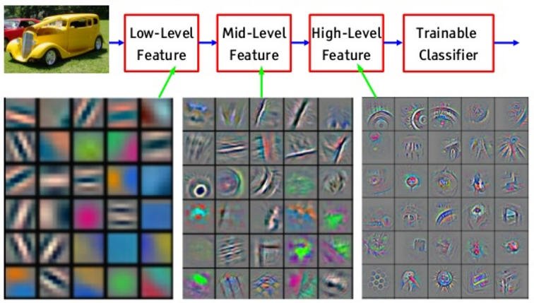
Hierarchy of features: I’ve mentioned the first convolutional layer. What about the ones above it? Those will recognize to recognize features based on features: they will combine basic features (vertical or horizontal lines, for example) into more and more general features: grids, parallel arrays, then objects from the real world composed of those features.

Hierarhcy of features

Environment

Our work will be made sweet and easy by Keras. Keras is just the kind of tool I love: it will let you do the most common operations quickly and easily, but it still gives you the power to go under the hood and have total control if you need it. It is a library built specifically for Deep Learning on Python by François Chollet and others. It runs on top of different backends, like Theano and Tensorflow. These are amazing libraries, but not the kind of thing that you want to deal with if you want to build your first prototype and iterate on it fast. You can think of the relationship between Keras and Tensorflow kind of like that between scikit-learn and numpy.

In order to follow the code below, you’ll need to set up a working Keras environment. The easiest way to do so is probably to use Google colab, a hosted notebook service which offers all relevant ML libraries preinstalled. They even offer free GPU acceleration! Just make sure you click on “runtime”/”change runtime type”, then select “GPU” before you run the notebooks. They also offer TPU acceleration for free! It’s a bit more involved, so we’ll just use GPUs for now.

At this point we want to get our first classifier up and running, so let’s get on with it!

import keras
from keras import backend as K

Using TensorFlow backend.

Getting some hotdogs

I’ve already done the hard, exhausting field work for you. If you are curious about how I did, check it out in the two previous installments, about imagenet and deep learning, and the train-test split.

In order to save you the trouble of downloading and cleaning, I have made the data available here. Run the following cell. It will download a zip file in the current folder.

!wget "https://www.dropbox.com/s/dhpekpce05iev6a/data_v2.zip?dl=0" -O data.zip

--2019-02-26 12:22:36--  https://www.dropbox.com/s/dhpekpce05iev6a/data_v2.zip?dl=0
Resolving www.dropbox.com (www.dropbox.com)... 162.125.65.1, 2620:100:6021:1::a27d:4101
Connecting to www.dropbox.com (www.dropbox.com)|162.125.65.1|:443... connected.
HTTP request sent, awaiting response... 301 Moved Permanently
Location: /s/raw/dhpekpce05iev6a/data_v2.zip [following]
--2019-02-26 12:22:37--  https://www.dropbox.com/s/raw/dhpekpce05iev6a/data_v2.zip
Reusing existing connection to www.dropbox.com:443.
HTTP request sent, awaiting response... 302 Found
Location: https://uc8e8a69e95e2f31d4d17093f3ef.dl.dropboxusercontent.com/cd/0/inline/AcES6X2ns7VwzQ7bV02YkEKzHGA7-UmuUQntl84McYrVl8ZM7f31B78QUWHmz-3-3bQJ4-muHv3qr3JRX2EaQSCEKr8KdjcUMlrP5Vosv9lV-nc2rb_HcSyMLPubn5KzG08/file# [following]
--2019-02-26 12:22:37--  https://uc8e8a69e95e2f31d4d17093f3ef.dl.dropboxusercontent.com/cd/0/inline/AcES6X2ns7VwzQ7bV02YkEKzHGA7-UmuUQntl84McYrVl8ZM7f31B78QUWHmz-3-3bQJ4-muHv3qr3JRX2EaQSCEKr8KdjcUMlrP5Vosv9lV-nc2rb_HcSyMLPubn5KzG08/file
Resolving uc8e8a69e95e2f31d4d17093f3ef.dl.dropboxusercontent.com (uc8e8a69e95e2f31d4d17093f3ef.dl.dropboxusercontent.com)... 162.125.65.6, 2620:100:6021:6::a27d:4106
Connecting to uc8e8a69e95e2f31d4d17093f3ef.dl.dropboxusercontent.com (uc8e8a69e95e2f31d4d17093f3ef.dl.dropboxusercontent.com)|162.125.65.6|:443... connected.
HTTP request sent, awaiting response... 302 FOUND
Location: /cd/0/inline2/AcErLUF0lUzNFsMdNcnh4bfAuYje6xpO1JE628_8xuBixqf_CEz9hz9mdxfPIhKy5jV0UtzidbGbyZsRY_F6_E9C7dfp1-vvyjasdQjGyD55weV7WwVxRcL8RUAxtrzZgBbGbmbfXz9bwBvO-WvArRgoVip3ddAMmYu9-rCFzfa68MkAlNb0Y2gZ59LPX8mf2ViJDTLwdu4AxmpTrEo8qCXedG769rAZ6pBGtg_IqOnlRZlXRDD4qY8JvVpNqwhLoOMPvoV-Kq0_CCAiiuXdPu7xSX9AJqhuXfnXGdxW59_tRbpRZSH6Waa84l2eexK_yuWXvgR-osxO5fKd6ZukL2GAvGdcPV9rsMZdtddimB2u0A/file [following]
--2019-02-26 12:22:38--  https://uc8e8a69e95e2f31d4d17093f3ef.dl.dropboxusercontent.com/cd/0/inline2/AcErLUF0lUzNFsMdNcnh4bfAuYje6xpO1JE628_8xuBixqf_CEz9hz9mdxfPIhKy5jV0UtzidbGbyZsRY_F6_E9C7dfp1-vvyjasdQjGyD55weV7WwVxRcL8RUAxtrzZgBbGbmbfXz9bwBvO-WvArRgoVip3ddAMmYu9-rCFzfa68MkAlNb0Y2gZ59LPX8mf2ViJDTLwdu4AxmpTrEo8qCXedG769rAZ6pBGtg_IqOnlRZlXRDD4qY8JvVpNqwhLoOMPvoV-Kq0_CCAiiuXdPu7xSX9AJqhuXfnXGdxW59_tRbpRZSH6Waa84l2eexK_yuWXvgR-osxO5fKd6ZukL2GAvGdcPV9rsMZdtddimB2u0A/file
Reusing existing connection to uc8e8a69e95e2f31d4d17093f3ef.dl.dropboxusercontent.com:443.
HTTP request sent, awaiting response... 200 OK
Length: 745085878 (711M) [application/zip]
Saving to: ‘data.zip’

data.zip            100%[===================>] 710.57M  45.2MB/s    in 17s     

2019-02-26 12:22:55 (41.2 MB/s) - ‘data.zip’ saved [745085878/745085878]

Now, unzip the zip file. It contains a ‘data’ folder that contains three folders in turn: train, test and validation. Inside each of those there are two folders: “hotdog” and “nohotdog”.

!rm -rf data/
!unzip -oq data.zip
!ls -lh data

total 12K
drwxrwxr-x 4 root root 4.0K Jun 27  2018 test
drwxrwxr-x 4 root root 4.0K Jun 27  2018 train
drwxrwxr-x 4 root root 4.0K Jun 27  2018 validation

Our first CNN

We are going to learn some hotdogs! The basic tool we are going to use is a Convolutional Neural Network (CNN). A CNN is easy to set up in Keras:

from keras.layers import Conv2D, MaxPooling2D, InputLayer, Flatten, Dense

my_first_cnn = keras.Sequential()
my_first_cnn.add(Conv2D(32, (3, 3), activation='relu', input_shape=(120, 120, 3)))
my_first_cnn.add(MaxPooling2D((2,2)))
my_first_cnn.add(Conv2D(32, (3, 3), activation='relu'))
my_first_cnn.add(MaxPooling2D((2,2)))
my_first_cnn.add(Flatten())
my_first_cnn.add(Dense(64, activation='relu'))
my_first_cnn.add(Dense(1, activation='sigmoid'))

my_first_cnn.summary()

WARNING:tensorflow:From /usr/local/lib/python3.6/dist-packages/tensorflow/python/framework/op_def_library.py:263: colocate_with (from tensorflow.python.framework.ops) is deprecated and will be removed in a future version.
Instructions for updating:
Colocations handled automatically by placer.
_________________________________________________________________
Layer (type)                 Output Shape              Param #   
=================================================================
conv2d_1 (Conv2D)            (None, 118, 118, 32)      896       
_________________________________________________________________
max_pooling2d_1 (MaxPooling2 (None, 59, 59, 32)        0         
_________________________________________________________________
conv2d_2 (Conv2D)            (None, 57, 57, 32)        9248      
_________________________________________________________________
max_pooling2d_2 (MaxPooling2 (None, 28, 28, 32)        0         
_________________________________________________________________
flatten_1 (Flatten)          (None, 25088)             0         
_________________________________________________________________
dense_1 (Dense)              (None, 64)                1605696   
_________________________________________________________________
dense_2 (Dense)              (None, 1)                 65        
=================================================================
Total params: 1,615,905
Trainable params: 1,615,905
Non-trainable params: 0
_________________________________________________________________

Now we need to feed the net. Create image data generators, which will give it regularly sized images in batches of the size we specify:

%%time
from keras.preprocessing.image import ImageDataGenerator
import os

base_dir = 'data//'

train_dir = os.path.join(base_dir, 'train')
validation_dir = os.path.join(base_dir, 'validation')

train_datagen = ImageDataGenerator(rescale=1 / 255)

test_datagen = ImageDataGenerator(rescale=1 / 255)

train_generator = train_datagen.flow_from_directory(train_dir, 
                                                    target_size=(120,120),
                                                    batch_size=100,
                                                    class_mode='binary')

validation_generator = test_datagen.flow_from_directory(validation_dir,
                                                        target_size=(120,120),
                                                        batch_size=100,
                                                        class_mode='binary')

Found 4765 images belonging to 2 classes.
Found 888 images belonging to 2 classes.
CPU times: user 167 ms, sys: 34.3 ms, total: 201 ms
Wall time: 320 ms

!ls data/validation/nohotdog | wc -l

And we are ready to train! We will need to “compile” the net, and fit it to the images our generators will provide:

%%time
from keras.optimizers import Adam

my_first_cnn.compile(loss='binary_crossentropy',
                     optimizer=Adam(lr=1e-3),
                     metrics=['acc'])

history = my_first_cnn.fit_generator(train_generator,
                                     steps_per_epoch=30,
                                     epochs=10,
                                     validation_data=validation_generator,
                                     validation_steps=10)

# Save the model. This can save us the trouble of retraining in later sessions.
my_first_cnn.save('my_first_cnn.h5')

WARNING:tensorflow:From /usr/local/lib/python3.6/dist-packages/tensorflow/python/ops/math_ops.py:3066: to_int32 (from tensorflow.python.ops.math_ops) is deprecated and will be removed in a future version.
Instructions for updating:
Use tf.cast instead.
Epoch 1/10
30/30 [==============================] - 22s 727ms/step - loss: 0.3967 - acc: 0.8747 - val_loss: 0.3128 - val_acc: 0.8694
Epoch 2/10
30/30 [==============================] - 19s 633ms/step - loss: 0.2876 - acc: 0.8761 - val_loss: 0.2927 - val_acc: 0.8694
Epoch 3/10
30/30 [==============================] - 19s 626ms/step - loss: 0.2561 - acc: 0.8797 - val_loss: 0.2520 - val_acc: 0.8755
Epoch 4/10
30/30 [==============================] - 19s 629ms/step - loss: 0.2473 - acc: 0.8734 - val_loss: 0.2527 - val_acc: 0.8694
Epoch 5/10
30/30 [==============================] - 19s 622ms/step - loss: 0.2537 - acc: 0.8731 - val_loss: 0.2336 - val_acc: 0.8796
Epoch 6/10
30/30 [==============================] - 19s 626ms/step - loss: 0.2260 - acc: 0.8787 - val_loss: 0.2521 - val_acc: 0.9059
Epoch 7/10
30/30 [==============================] - 18s 599ms/step - loss: 0.2075 - acc: 0.8954 - val_loss: 0.2272 - val_acc: 0.8968
Epoch 8/10
30/30 [==============================] - 19s 638ms/step - loss: 0.2043 - acc: 0.8962 - val_loss: 0.2218 - val_acc: 0.9028
Epoch 9/10
30/30 [==============================] - 19s 619ms/step - loss: 0.1690 - acc: 0.9123 - val_loss: 0.2489 - val_acc: 0.8863
Epoch 10/10
30/30 [==============================] - 18s 610ms/step - loss: 0.1956 - acc: 0.9046 - val_loss: 0.2412 - val_acc: 0.8968
CPU times: user 4min 34s, sys: 8.73 s, total: 4min 42s
Wall time: 3min 10s

Magic! In only a few minutes, we are getting a classifier with close to 90% accuracy! Time to celebrate!

Party!

Let’s go to bed with that sweet sweet feeling. Future Dani will take care of the cleanup. I’m sure everything is well and good with our classifier.

Or is it not? We will take a closer look at how well it performs in the next installment.