
Sometimes, getting more data is not an option. But it need not spell doom for your Deep Learning project. There is a technique that can help you make the most of limited data. It’s called [Data augmentation] and that’s what I’ll talk about today. This is part 5 of a series on Deep Learning. You can can find parts 1-4 in the following links:
You can execute the code in this notebook by clicking the following:
![]()
Hi there! Welcome back to my gentle introduction to Deep Learning. With hot dogs.
Last time we finally got our first actual taste of what Deep Learning, and specifically ConvNets, are. We got a decent classifier, but it’s still far from production ready. Jian-Yang is proud, but the Periscope guys are not impressed. We need a better classifier so that we can sell the company to them and become really rich.
There are many different techniques that you can apply to an image classifier that does not perform as well as necessary. The most powerful, and the most obvious, is to get more data (pdf link). A simple model with a lot of data will most of the time outperform a more complex model with little data.
However, enlarging our data set is not always possible, and most of the time it is actually pretty expensive, either in terms of money or time. I’m not about to go out and spend a few weeks photographing hot dogs!
What if we could make the data up? Well, for a certain definition of “making up”, we can. It actually makes a lot of sense and can improve performance quite a bit. Think about it: our sample images each represent just one possible view of the hotdog. Our classifier can get hung up on minor details that would not be so apparent if the hotdog was partially cropped or distorted, so if we show it modified images on top of the ones we already have we will both have more images and a more generalizable classifier!
Data augmentation
The idea is simple: we don’t have that many images, specially of hotdogs, so let’s make the most of the few we have. We’ll generate new images by applying a number of transformations to the ones we have: we will zoom in, out, distort them a bit, translate them, rotate them…
Luckily, we basically don’t have to code any of this: it’s already provided by the ImageDataGenerator class in Keras!
# Delete this line if you are not running the notebook in colab
%tensorflow_version 1.x
# Silence some annoying deprecation warnings
import logging
logging.getLogger('tensorflow').disabled = True

import keras
from keras.preprocessing.image import ImageDataGenerator
from keras.layers import Conv2D, MaxPooling2D, InputLayer, Flatten, Dense
from keras.optimizers import Adam
import os

# Download the data
!wget -q "https://www.dropbox.com/s/dhpekpce05iev6a/data_v2.zip?dl=0" -O data.zip
!rm -rf data/
!unzip -oq data.zip
!ls -lh data
base_dir = 'data/'

train_dir = os.path.join(base_dir, 'train')
validation_dir = os.path.join(base_dir, 'validation')

train_datagen = ImageDataGenerator(rescale=1 / 255,
                                   rotation_range=40,
                                   width_shift_range=0.2,
                                   height_shift_range=0.2,
                                   shear_range=0.2,
                                   zoom_range=0.2,
                                   horizontal_flip=True,
                                   fill_mode='nearest')

test_datagen = ImageDataGenerator(rescale=1 / 255)
Using TensorFlow backend.
It’s important to only apply this to the training generator: we don’t want to be transforming the validation set, since we want it to be reflective of the kinds of images we might find in the wild.
train_generator = train_datagen.flow_from_directory(train_dir,
                                                    target_size=(120,120),
                                                    batch_size=100,
                                                    class_mode='binary')

validation_generator = test_datagen.flow_from_directory(validation_dir,
                                                        target_size=(120,120),
                                                        batch_size=100,
                                                        class_mode='binary')

validation_generator_noshuffle = test_datagen.flow_from_directory(validation_dir,
                                                        target_size=(120,120),
                                                        batch_size=100,
                                                        shuffle=False,
                                                        class_mode='binary')
Found 4765 images belonging to 2 classes.
Found 888 images belonging to 2 classes.
Found 888 images belonging to 2 classes.
my_2nd_cnn = keras.Sequential()
my_2nd_cnn.add(Conv2D(32, (3, 3), activation='relu', input_shape=(120, 120, 3)))
my_2nd_cnn.add(MaxPooling2D((2,2)))
my_2nd_cnn.add(Conv2D(32, (3, 3), activation='relu'))
my_2nd_cnn.add(MaxPooling2D((2,2)))
my_2nd_cnn.add(Flatten())
my_2nd_cnn.add(Dense(64, activation='relu'))
my_2nd_cnn.add(Dense(1, activation='sigmoid'))

my_2nd_cnn.summary()
_________________________________________________________________
Layer (type)                 Output Shape              Param #
=================================================================
conv2d_1 (Conv2D)            (None, 118, 118, 32)      896
_________________________________________________________________
max_pooling2d_1 (MaxPooling2 (None, 59, 59, 32)        0
_________________________________________________________________
conv2d_2 (Conv2D)            (None, 57, 57, 32)        9248
_________________________________________________________________
max_pooling2d_2 (MaxPooling2 (None, 28, 28, 32)        0
_________________________________________________________________
flatten_1 (Flatten)          (None, 25088)             0
_________________________________________________________________
dense_1 (Dense)              (None, 64)                1605696
_________________________________________________________________
dense_2 (Dense)              (None, 1)                 65
=================================================================
Total params: 1,615,905
Trainable params: 1,615,905
Non-trainable params: 0
_________________________________________________________________
%%time
my_2nd_cnn.compile(loss='binary_crossentropy',
                   optimizer=Adam(lr=1e-3),
                   metrics=['acc'])

history = my_2nd_cnn.fit_generator(train_generator,
                                   class_weight = {0: 7, 1: 1},
                                   steps_per_epoch=30,
                                   epochs=25,
                                   validation_data=validation_generator,
                                   validation_steps=10,
                                   verbose=1)
Epoch 1/25
30/30 [==============================] - 122s 4s/step - loss: 1.0534 - acc: 0.6815 - val_loss: 0.4138 - val_acc: 0.8553
Epoch 2/25
30/30 [==============================] - 20s 673ms/step - loss: 0.8585 - acc: 0.7837 - val_loss: 0.6537 - val_acc: 0.7065
Epoch 3/25
30/30 [==============================] - 20s 656ms/step - loss: 0.8202 - acc: 0.7708 - val_loss: 0.4769 - val_acc: 0.7804
Epoch 4/25
30/30 [==============================] - 20s 673ms/step - loss: 0.6956 - acc: 0.8173 - val_loss: 0.3017 - val_acc: 0.8593
Epoch 5/25
30/30 [==============================] - 20s 674ms/step - loss: 0.7376 - acc: 0.7886 - val_loss: 0.3053 - val_acc: 0.8654
Epoch 6/25
30/30 [==============================] - 20s 657ms/step - loss: 0.6671 - acc: 0.8192 - val_loss: 0.4276 - val_acc: 0.8117
Epoch 7/25
30/30 [==============================] - 20s 652ms/step - loss: 0.7145 - acc: 0.8023 - val_loss: 0.3390 - val_acc: 0.8492
Epoch 8/25
30/30 [==============================] - 20s 682ms/step - loss: 0.7007 - acc: 0.8150 - val_loss: 0.2340 - val_acc: 0.9049
Epoch 9/25
30/30 [==============================] - 20s 664ms/step - loss: 0.6074 - acc: 0.8295 - val_loss: 0.3102 - val_acc: 0.8573
Epoch 10/25
30/30 [==============================] - 20s 674ms/step - loss: 0.6938 - acc: 0.8210 - val_loss: 0.3605 - val_acc: 0.8219
Epoch 11/25
30/30 [==============================] - 19s 644ms/step - loss: 0.6704 - acc: 0.8147 - val_loss: 0.3172 - val_acc: 0.8502
Epoch 12/25
30/30 [==============================] - 20s 658ms/step - loss: 0.6680 - acc: 0.8350 - val_loss: 0.3024 - val_acc: 0.8715
Epoch 13/25
30/30 [==============================] - 20s 673ms/step - loss: 0.6101 - acc: 0.8400 - val_loss: 0.2766 - val_acc: 0.8664
Epoch 14/25
30/30 [==============================] - 20s 652ms/step - loss: 0.5874 - acc: 0.8340 - val_loss: 0.2676 - val_acc: 0.8745
Epoch 15/25
30/30 [==============================] - 20s 672ms/step - loss: 0.6006 - acc: 0.8500 - val_loss: 0.2819 - val_acc: 0.8704
Epoch 16/25
30/30 [==============================] - 20s 665ms/step - loss: 0.5845 - acc: 0.8367 - val_loss: 0.3057 - val_acc: 0.8553
Epoch 17/25
30/30 [==============================] - 20s 665ms/step - loss: 0.5494 - acc: 0.8458 - val_loss: 0.3038 - val_acc: 0.8431
Epoch 18/25
30/30 [==============================] - 20s 676ms/step - loss: 0.6681 - acc: 0.8210 - val_loss: 0.4019 - val_acc: 0.8117
Epoch 19/25
30/30 [==============================] - 20s 655ms/step - loss: 0.6010 - acc: 0.8279 - val_loss: 0.2798 - val_acc: 0.8715
Epoch 20/25
30/30 [==============================] - 20s 678ms/step - loss: 0.6289 - acc: 0.8220 - val_loss: 0.2986 - val_acc: 0.8512
Epoch 21/25
30/30 [==============================] - 20s 664ms/step - loss: 0.7047 - acc: 0.8126 - val_loss: 0.4141 - val_acc: 0.8158
Epoch 22/25
30/30 [==============================] - 20s 668ms/step - loss: 0.5445 - acc: 0.8517 - val_loss: 0.2840 - val_acc: 0.8725
Epoch 23/25
30/30 [==============================] - 20s 675ms/step - loss: 0.5534 - acc: 0.8453 - val_loss: 0.2294 - val_acc: 0.9028
Epoch 24/25
30/30 [==============================] - 20s 661ms/step - loss: 0.5636 - acc: 0.8519 - val_loss: 0.3119 - val_acc: 0.8532
Epoch 25/25
30/30 [==============================] - 20s 663ms/step - loss: 0.6476 - acc: 0.8239 - val_loss: 0.3966 - val_acc: 0.8209
from mateosio import plot_training_histories
%matplotlib inline
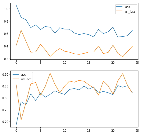
plot_training_histories(history);
from mateosio import plot_confusion_matrix
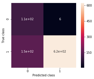
ax, precision, recall = plot_confusion_matrix(my_2nd_cnn, validation_generator_noshuffle)
print(precision, recall)
0.415384615385 0.947368421053
Wow, now I am underfitting! I guess that means I can make my model even a bit more complex, let’s see.
One more layer
my_3rd_cnn = keras.Sequential()
my_3rd_cnn.add(Conv2D(32, (3, 3), activation='relu', input_shape=(120, 120, 3)))
my_3rd_cnn.add(MaxPooling2D((2,2)))
my_3rd_cnn.add(Conv2D(32, (3, 3), activation='relu'))
my_3rd_cnn.add(MaxPooling2D((2,2)))
my_3rd_cnn.add(Flatten())
my_3rd_cnn.add(Dense(128, activation='relu'))
my_3rd_cnn.add(Dense(128, activation='relu'))
my_3rd_cnn.add(Dense(64, activation='relu'))
my_3rd_cnn.add(Dense(1, activation='sigmoid'))

my_3rd_cnn.summary()
_________________________________________________________________
Layer (type)                 Output Shape              Param #
=================================================================
conv2d_3 (Conv2D)            (None, 118, 118, 32)      896
_________________________________________________________________
max_pooling2d_3 (MaxPooling2 (None, 59, 59, 32)        0
_________________________________________________________________
conv2d_4 (Conv2D)            (None, 57, 57, 32)        9248
_________________________________________________________________
max_pooling2d_4 (MaxPooling2 (None, 28, 28, 32)        0
_________________________________________________________________
flatten_2 (Flatten)          (None, 25088)             0
_________________________________________________________________
dense_3 (Dense)              (None, 128)               3211392
_________________________________________________________________
dense_4 (Dense)              (None, 128)               16512
_________________________________________________________________
dense_5 (Dense)              (None, 64)                8256
_________________________________________________________________
dense_6 (Dense)              (None, 1)                 65
=================================================================
Total params: 3,246,369
Trainable params: 3,246,369
Non-trainable params: 0
_________________________________________________________________
%%time
my_3rd_cnn.compile(loss='binary_crossentropy',
                   optimizer=Adam(lr=1e-3),
                   metrics=['acc'])

history = my_3rd_cnn.fit_generator(train_generator,
                                   class_weight = {0: 7, 1: 1},
                                   steps_per_epoch=30,
                                   epochs=20,
                                   validation_data=validation_generator,
                                   validation_steps=10,
                                   verbose=1)
Epoch 1/20
30/30 [==============================] - 23s 773ms/step - loss: 1.0655 - acc: 0.6366 - val_loss: 0.4718 - val_acc: 0.7561
Epoch 2/20
30/30 [==============================] - 20s 664ms/step - loss: 0.8330 - acc: 0.7680 - val_loss: 0.8183 - val_acc: 0.5729
Epoch 3/20
30/30 [==============================] - 20s 676ms/step - loss: 0.7935 - acc: 0.7830 - val_loss: 0.5478 - val_acc: 0.6953
Epoch 4/20
30/30 [==============================] - 20s 669ms/step - loss: 0.7688 - acc: 0.7760 - val_loss: 0.2606 - val_acc: 0.8988
Epoch 5/20
30/30 [==============================] - 20s 671ms/step - loss: 0.7634 - acc: 0.7770 - val_loss: 0.3780 - val_acc: 0.8117
Epoch 6/20
30/30 [==============================] - 20s 668ms/step - loss: 0.7331 - acc: 0.7857 - val_loss: 0.3855 - val_acc: 0.8138
Epoch 7/20
30/30 [==============================] - 20s 660ms/step - loss: 0.7614 - acc: 0.8078 - val_loss: 0.3675 - val_acc: 0.8360
Epoch 8/20
30/30 [==============================] - 20s 666ms/step - loss: 0.6590 - acc: 0.8107 - val_loss: 0.4328 - val_acc: 0.7763
Epoch 9/20
30/30 [==============================] - 20s 679ms/step - loss: 0.7267 - acc: 0.7827 - val_loss: 0.4281 - val_acc: 0.7672
Epoch 10/20
30/30 [==============================] - 20s 665ms/step - loss: 0.6466 - acc: 0.7999 - val_loss: 0.4618 - val_acc: 0.7338
Epoch 11/20
30/30 [==============================] - 21s 686ms/step - loss: 0.6373 - acc: 0.8013 - val_loss: 0.2889 - val_acc: 0.8917
Epoch 12/20
30/30 [==============================] - 20s 660ms/step - loss: 0.6980 - acc: 0.8059 - val_loss: 0.4655 - val_acc: 0.7773
Epoch 13/20
30/30 [==============================] - 20s 663ms/step - loss: 0.6496 - acc: 0.8003 - val_loss: 0.2856 - val_acc: 0.8573
Epoch 14/20
30/30 [==============================] - 20s 673ms/step - loss: 0.6660 - acc: 0.7937 - val_loss: 0.3241 - val_acc: 0.8340
Epoch 15/20
30/30 [==============================] - 20s 676ms/step - loss: 0.6411 - acc: 0.8110 - val_loss: 0.3288 - val_acc: 0.8391
Epoch 16/20
30/30 [==============================] - 20s 660ms/step - loss: 0.6320 - acc: 0.8220 - val_loss: 0.3424 - val_acc: 0.8239
Epoch 17/20
30/30 [==============================] - 20s 678ms/step - loss: 0.6161 - acc: 0.8260 - val_loss: 0.3175 - val_acc: 0.8411
Epoch 18/20
30/30 [==============================] - 20s 662ms/step - loss: 0.6798 - acc: 0.8035 - val_loss: 0.3317 - val_acc: 0.8310
Epoch 19/20
30/30 [==============================] - 20s 655ms/step - loss: 0.5905 - acc: 0.8302 - val_loss: 0.3413 - val_acc: 0.8401
Epoch 20/20
30/30 [==============================] - 20s 661ms/step - loss: 0.6207 - acc: 0.8241 - val_loss: 0.2859 - val_acc: 0.8775
plot_training_histories(history);
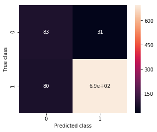
ax, precision, recall = plot_confusion_matrix(my_3rd_cnn, validation_generator_noshuffle)
print(precision, recall)
0.509202453988 0.728070175439
One of the best pieces of advice I got from Jeremy Howard’s Deep Learning for Coders is that you should first attempt to overfit, then deal with that through regularization. It makes a lot of sense: once you have overfitting, you know you’ve juiced your model to the max. If you don’t, you don’t know whether there is still a lot of life left on it or it’s at the maximum performance it’s going to get. Let’s go for that overfitting.
Once a model stops improving with a particular learning rate, it’s often useful to reduce the learning rate and keep training.
%%time
my_3rd_cnn.compile(loss='binary_crossentropy',
                   optimizer=Adam(lr=1e-4),
                   metrics=['acc'])

history_pt2 = my_3rd_cnn.fit_generator(train_generator,
                                       class_weight = {0: 7, 1: 1},
                                       steps_per_epoch=30,
                                       epochs=30,
                                       validation_data=validation_generator,
                                       validation_steps=10,
                                       verbose=1)
Epoch 1/30
30/30 [==============================] - 23s 774ms/step - loss: 0.6566 - acc: 0.7980 - val_loss: 0.2879 - val_acc: 0.8573
Epoch 2/30
30/30 [==============================] - 20s 671ms/step - loss: 0.5584 - acc: 0.8387 - val_loss: 0.3417 - val_acc: 0.8289
Epoch 3/30
30/30 [==============================] - 20s 660ms/step - loss: 0.5600 - acc: 0.8425 - val_loss: 0.3182 - val_acc: 0.8320
Epoch 4/30
30/30 [==============================] - 20s 667ms/step - loss: 0.5453 - acc: 0.8314 - val_loss: 0.3467 - val_acc: 0.8330
Epoch 5/30
30/30 [==============================] - 20s 680ms/step - loss: 0.5742 - acc: 0.8280 - val_loss: 0.3430 - val_acc: 0.8259
Epoch 6/30
30/30 [==============================] - 20s 658ms/step - loss: 0.5122 - acc: 0.8405 - val_loss: 0.2929 - val_acc: 0.8623
Epoch 7/30
30/30 [==============================] - 20s 669ms/step - loss: 0.5503 - acc: 0.8429 - val_loss: 0.3180 - val_acc: 0.8512
Epoch 8/30
30/30 [==============================] - 21s 683ms/step - loss: 0.5481 - acc: 0.8373 - val_loss: 0.2798 - val_acc: 0.8704
Epoch 9/30
30/30 [==============================] - 20s 652ms/step - loss: 0.5973 - acc: 0.8335 - val_loss: 0.3123 - val_acc: 0.8462
Epoch 10/30
30/30 [==============================] - 20s 671ms/step - loss: 0.5306 - acc: 0.8440 - val_loss: 0.2748 - val_acc: 0.8735
Epoch 11/30
30/30 [==============================] - 20s 672ms/step - loss: 0.5613 - acc: 0.8360 - val_loss: 0.3041 - val_acc: 0.8603
Epoch 12/30
30/30 [==============================] - 20s 663ms/step - loss: 0.5303 - acc: 0.8483 - val_loss: 0.2930 - val_acc: 0.8583
Epoch 13/30
30/30 [==============================] - 20s 681ms/step - loss: 0.5578 - acc: 0.8399 - val_loss: 0.3194 - val_acc: 0.8462
Epoch 14/30
30/30 [==============================] - 20s 656ms/step - loss: 0.5664 - acc: 0.8387 - val_loss: 0.2919 - val_acc: 0.8603
Epoch 15/30
30/30 [==============================] - 20s 681ms/step - loss: 0.5157 - acc: 0.8550 - val_loss: 0.3484 - val_acc: 0.8269
Epoch 16/30
30/30 [==============================] - 20s 664ms/step - loss: 0.5506 - acc: 0.8413 - val_loss: 0.2914 - val_acc: 0.8532
Epoch 17/30
30/30 [==============================] - 20s 675ms/step - loss: 0.5222 - acc: 0.8423 - val_loss: 0.3223 - val_acc: 0.8462
Epoch 18/30
30/30 [==============================] - 20s 665ms/step - loss: 0.5332 - acc: 0.8515 - val_loss: 0.3179 - val_acc: 0.8441
Epoch 19/30
30/30 [==============================] - 20s 651ms/step - loss: 0.5383 - acc: 0.8521 - val_loss: 0.3342 - val_acc: 0.8421
Epoch 20/30
30/30 [==============================] - 20s 674ms/step - loss: 0.5421 - acc: 0.8432 - val_loss: 0.3227 - val_acc: 0.8391
Epoch 21/30
30/30 [==============================] - 20s 664ms/step - loss: 0.5345 - acc: 0.8463 - val_loss: 0.3051 - val_acc: 0.8563
Epoch 22/30
30/30 [==============================] - 20s 670ms/step - loss: 0.5444 - acc: 0.8479 - val_loss: 0.3302 - val_acc: 0.8411
Epoch 23/30
30/30 [==============================] - 20s 660ms/step - loss: 0.4902 - acc: 0.8537 - val_loss: 0.2945 - val_acc: 0.8573
Epoch 24/30
30/30 [==============================] - 20s 666ms/step - loss: 0.5113 - acc: 0.8559 - val_loss: 0.2703 - val_acc: 0.8755
Epoch 25/30
30/30 [==============================] - 20s 673ms/step - loss: 0.5130 - acc: 0.8480 - val_loss: 0.2724 - val_acc: 0.8644
Epoch 26/30
30/30 [==============================] - 20s 658ms/step - loss: 0.4878 - acc: 0.8580 - val_loss: 0.2768 - val_acc: 0.8664
Epoch 27/30
30/30 [==============================] - 20s 668ms/step - loss: 0.4796 - acc: 0.8626 - val_loss: 0.2604 - val_acc: 0.8887
Epoch 28/30
30/30 [==============================] - 21s 689ms/step - loss: 0.5074 - acc: 0.8470 - val_loss: 0.2908 - val_acc: 0.8704
Epoch 29/30
30/30 [==============================] - 20s 683ms/step - loss: 0.5374 - acc: 0.8515 - val_loss: 0.3367 - val_acc: 0.8401
Epoch 30/30
30/30 [==============================] - 20s 655ms/step - loss: 0.5458 - acc: 0.8377 - val_loss: 0.2894 - val_acc: 0.8573
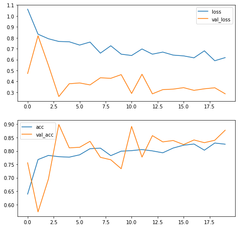
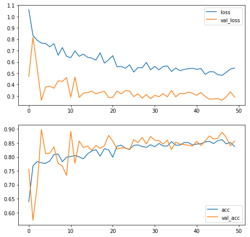
plot_training_histories(history, history_pt2);
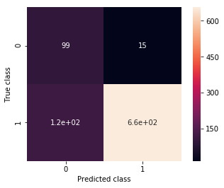
ax, precision, recall = plot_confusion_matrix(my_3rd_cnn, validation_generator_noshuffle)
print(precision, recall)
0.456221198157 0.868421052632
Great! We have improved quite a lot! Even better, judging by the loss/validation plot we have still quite a way to go in making the model better. However, in what direction should we take it? More fully connected layers? More convolutional ones? The possibility space is endless, so it’s hard to say. Additionally, the more complex we make the model, the more parameters we’ll have to train.
Turns out, there’s a technique that sidesteps both potential problems. I’ll show it to you in the next episode!
Further Reading
Deep Learning with Python: A great introductory book by François Chollet, author of Keras. Explains the practice first, then goes down to theory.
fast.ai’s course image classification part: Very good course for learning the concepts, even if they insist in using their own library.